We invite you to download (freely) our ptychographic reconstruction algorithm for SHG frequency resolved optical gating (FROG). The new reconstruction method exhibits several useful features including robustness to noise and the possibility for super-resolution.
You may read our paper: Ptychographic reconstruction algorithm for frequency resolved optical gating: super-resolution and supreme robustness.
The reconstruction algorithm is based on extended Ptychographical Iterative Engine (ePIE) which is used in ptychography. We modified it for pulse reconstruction from FROG traces and also discovered that ptychography can yield super-resolution directly, without any hardware modifications or assumption about the probed signal.
The algorithm allows retrieving the complex pulses from a very small number of delay steps and/or from a spectrally incomplete FROG trace because, in contrast to current general projections (GP) algorithms, the ptychographical approach does not couple between the spectral and delay axes.
You are most welcome to send us your comments/suggestions/feedback.
- Download zip archive ptych_FROG.zip or PG_FROG.zip and unpack all files to the same directory
- Inside the archive you will find the following files:
pulse_set.mat – Bank of 100 random pulses
ePIE_fun_FROG.m – MATLAB implementation of the ptychographic SHG FROG algorithm without any prior information about the pulse.
ePIE_fun_FROG_sp.m – MATLAB implementation of the ptychographic SHG FROG algorithm, which employs prior knowledge about the pulse power spectrum.
best_sol.m - is a function that removes trivial ambiguities between reference and reconstructed pulses.
main_simulator.m - is a script that loads a bank of 100 random pulses, chooses one of them, produces corresponding FROG trace (with or without spectral filter) and reconstructs the pulse from the FROG trace. - Running main_simulator.m, you should get the following figure:
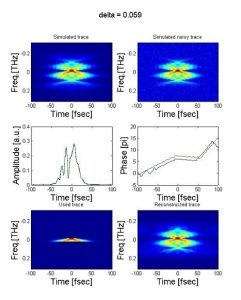
- In main_simulator.m, you can choose the reconstruction algorithm without any prior information about the pulse, in this case use alg=1, (line 12). Write alg=2, (line 12) in order to take into account the known power spectrum of the pulse.
- In order to apply the reconstruction code on your generated pulse, insert it to the vector ‘pulse’ in
line 16 in main_simulator.m - ‘LPF_flag’ in line 14 in main_simulator.m turns the spectral low pass filter on/off, with cutoff frequency that is controlled by ‘Fsupp’ in line 29 in main_simulator.m.
- The level of noise applied to the FROG trace is determined in line 26 of main_simulator.m.